Parity Challenge Solution

The article details the solution provided by the winner of the Parity challenge.

Author: Chi-Hieu Nguyen, University of Technology Sydney, Australia.

Overview of the approach

The parity function $parity(x) = x \mod 2$ is intimately connected to the bit extraction problem, where the goal is to determine the bit representation of a given integer $x$ the goal such that $x=\sum2^ib_i$. This function can be expressed in the continuous domain using the trigonometric function $f: [0,255] \to [0,1],\; f(x) = \frac{1}{2}(\cos(\pi (x+1))+1)$. Evaluating trigonometric functions in an encrypted domain is a well-established problem, which is frequently employed in the bootstrapping process to refresh the level of an "exhausted" ciphertext [1]. A common approach to evaluating a cosine function is to utilize the double-angle formula $\cos(2x)=2\cos^2x-1$ to evaluate $\cos(2x)$ from an approximation of $\cos(x)$, thus narrowing down the approximation range and reduce the order of the approximated polynomial.

We adopt the same approach and try to approximate $f$ using Chebyshev basis. Initially, the input value $x$ is normalized to the interval $[-1,1]$ using the linear transformation $y = \frac{x-128}{128}$. The target function becomes $f: [-1,1] \to [0,1],\; f(y) = \frac{1}{2}(\cos(\pi(128y+129))+1)=\frac{1}{2}(\cos(128\pi y+\pi)+1)$. Using the double angle formula, we first approximate $\cos\left(\pi y+\frac{\pi}{128}\right)$ by a polynomial $p(y)$ and then apply the transformation $h(y) = 2y^2-1$ to iteratively calculate $(h^7\circ p)(y)$, which approximates $\cos\left(128\pi y+\pi\right)$. The approximation of $\cos\left(\pi y+\frac{\pi}{128}\right)$ can be obtained using the numpy.polyfit method in Python.

f = lambda x: np.cos(np.pi*x+np.pi/128)
x = np.arange(0,257)
y = (x-128)/128
p = np.polyfit(y, f(y), 8)

This method returns a list of coefficients in the monomial basis, which must be converted to the Chebyshev basis for stable evaluation in a fixed-point environment. Figure 1 shows an illustration of such approximation using a polynomial of degree 8.

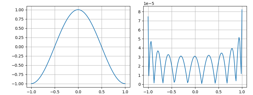
Figure 1: (left) Approximation of $\cos\left(\pi y+\frac{\pi}{128}\right)$ using an 8th-degree polynomial. (right) Absolute error of the approximation.

The interpolant appears accurate at this stage. However, after applying the double-angle iteration 7 times, the accuracy degrades beyond the desired bounds. Figure 2 depicts the resulting approximation, showing significant errors at certain values (e.g., $0, 126, 127, 128, 255, 256$) that exceed the acceptable threshold of $0.01$.

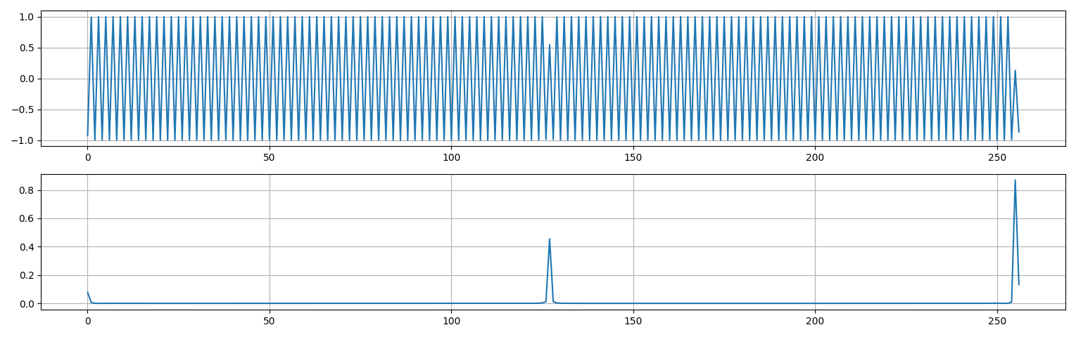
Figure 2: (top) Approximation of $\cos\left(128\pi y+\pi\right)$ after 7 double angle iterations. (bottom) Absolute error of the approximation.

To address this issue, we refined the polynomial approximation using a modified Arnoldi method as introduced in [2]. Unlike the referenced approach, which uses the error $\left|p(y) - \cos\left(\pi y+\frac{\pi}{128}\right)\right|$, we utilize the final error after the 7th double-angle iteration to update the weight vector for next steps. The Python code for improving the polynomial approximation is as follows:

g = lambda x: np.cos(128*np.pi*x+np.pi)
w = np.ones_like(y)
for _ in range(5):
    p = np.polyfit(y, f(y), 8, w=np.sqrt(w))
    z = np.polyval(p,y)
    for i in range(7):
        z = 2*z*z-1

    w = w*np.abs(z-g(y))
    w = w / np.linalg.norm(w)
    w = np.abs(w)

After 5 iterations, the maximum approximation error reduced to below $3\times 10^{-4}$, indicating a satisfactory solution. Figure 3 presents the final approximation.

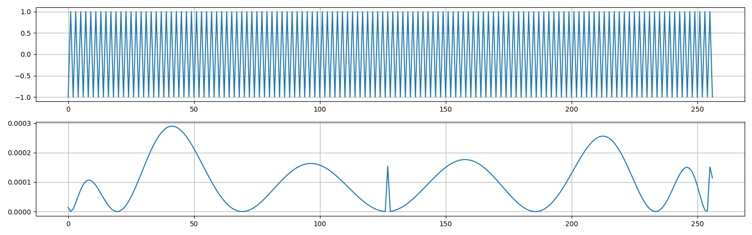
Figure 3: (top) The final approximation. (bottom) Absolute error of the approximation.

We can now convert the resulting polynomial to Chebyshev basis for evaluation.

print(np.polynomial.chebyshev.poly2cheb(p[::-1]))
# [-3.04159700e-01 -1.39659316e-02 -9.70590161e-01  1.63649478e-02
#   3.02827581e-01 -2.56364745e-03 -2.91082990e-02  1.66592418e-04
#   1.33270778e-03]

Optimizations

To further accelerate the polynomial evaluation, we apply a simple input-shifting trick. That is, instead of directly approximating $\cos\left(\pi y+\frac{\pi}{128}\right)$, we approximate $p(y) \approx \cos\left(\pi y\right)$ using the same method and then evaluate $p\left(y+\frac{\pi}{128}\right)$ to obtain $\cos\left(\pi y+\frac{\pi}{128}\right)$. Since $\cos\left(\pi y\right)$ is an even function, its Chebyshev representation contains only even-degree terms, allowing us to omit the odd-degree terms for faster evaluation. The updated Chebyshev representation of $p$ is as follows.

# [-0.3042513777371315, 0, -0.970882602838183, 0, 0.30291864798067064, 0, -0.02911740974995488, 0, 0.0013327077835582305]

Finally, recall that our the target function is $f(y) = \frac{1}{2}(\cos(128\pi y+\pi)+1)$, the approximation of $\cos(128\pi y+\pi)$ must be scaled by $\frac{1}{2}$, which inccurs an extra multiplication level. To avoid this, we scale the coefficients of $p$ by $\frac{2}{\sqrt[2^7]{4}}$ to approximate $\frac{2}{\sqrt[2^7]{4}}\cos\left(\pi y\right)$. We then apply a serie of transformation $h_i(y) = y^2-2\left(\frac{1}{\sqrt[2^7]{4}}\right)^{2^i}$ to calculate $(h_7\circ \cdots \circ h_1\circ p)\left(y+\frac{\pi}{128}\right) \approx \frac{1}{2}\cos(128\pi y+\pi)$. The final approximation of $f(y)$ is obtained by adding $\frac{1}{2}$ to the resulting value. The multiplication depth of the whole computation is 12 (1 for evaluating $y$, 4 for evaluating $p(y)$ and 7 for the transformations $h_1,\dots,h_7$).

References

[1] J.-P. Bossuat, C. Mouchet, J. Troncoso-Pastoriza and A.-P. Hubaux, "Efficient bootstrapping for approximate homomorphic encryption with non-sparse keys", Proc. EUROCRYPT, pp. 587-617, 2021.

[2] Pablo D Brubeck, Yuji Nakatsukasa, and Lloyd N Trefethen, "Vandermonde with Arnoldi", SIAM Review, 63(2):405–415, 2021.